Within scikit-learn, pipelines allow for the consolidation of all data preprocessing steps along with a final estimator using a single interface. The pipeline object can then be passed into a grid search routine to identify optimal hyperparameters. According to the documentation, the purpose of the pipeline is to assemble several steps that can be cross-validated together while setting different parameters. In this post, we’ll demonstrate how to utilize pipelines to preprocess the adult income data set and fit two classifiers to determine whether a given observation has an income in excess of $50,000 given the set of associated features. We first read in the data and inspect the first few records:
   age  workclass  fnlwgt     education  educational-num      marital-status         occupation relationship   race  gender  capital-gain  capital-loss  hours-per-week native-country income
0   25    Private  226802          11th                7       Never-married  Machine-op-inspct    Own-child  Black    Male             0             0              40  United-States  <=50K
1   38    Private   89814       HS-grad                9  Married-civ-spouse    Farming-fishing      Husband  White    Male             0             0              50  United-States  <=50K
2   28  Local-gov  336951    Assoc-acdm               12  Married-civ-spouse    Protective-serv      Husband  White    Male             0             0              40  United-States   >50K
3   44    Private  160323  Some-college               10  Married-civ-spouse  Machine-op-inspct      Husband  Black    Male          7688             0              40  United-States   >50K
4   18          ?  103497  Some-college               10       Never-married                  ?    Own-child  White  Female             0             0              30  United-States  <=50K
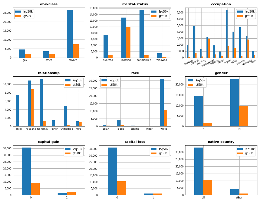
After loading the dataset, the first task is to get an idea of the frequency of different groups within categorical features. In the next cell, a dictionary is created for each categorical feature which remaps groups to ensure a reasonable number of observations in each:
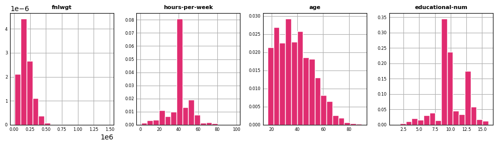
Next we distinguish between categorical and continuous features. Categorical features are re-mapped to align with the groups defined above. For categorical features, we assign null values to a “missing” category instead of relying on an imputation rule. This allows us to check for possible patterns in the missing data later on. capital-gain and capital-loss are converted into binary indicators and native-country into US vs. non-US. Finally, we split the data into training and validation sets ensuring the same proportion of positive instances in each cut:
We are now in a position to create our pipelines. The first pipeline is created to support a logistic regression classifier. We initialize a ColumnTransformer instance, which gives us the ability to define separate preprocessing steps for different groups of columns (in our case, categorical vs. continuous). As the logistic regression classifier doesn’t support categorical features, we one-hot encode them. In addition, since the logistic regression classifier relies on gradient descent to estimate coefficients, continuous features are scaled using RobustScaler to help with convergence and missing values imputed using IterativeImputer. For the classifier, we use the elasticnet penalty, which is a blend of lasso and ridge penalties. We’ll determine the optimal weighting using grid search.
Notice that set_output is affixed to pipeline1 by specifying transform="pandas". This was added in scikit-learn version 1.2, and allows intermediate and final datasets to be represented as Pandas DataFrames instead of Numpy arrays. I’ve found this to be particularly convenient, especially when inspecting the results of a transformation.
A different set of preprocessing steps is carried out for the HistGradientBoostingClassifier instance, which is functionally equivalent to lightgbm. Since HistGradientBoostingClassifier supports categorical features, it isn’t necessary to one-hot encode: We pass a list of columns that should be treated as nominal categorical features to the categorical_features parameter. Coming out of ColumnTransformer, categorical features are renamed with a leading categorical__, so it is easy to identify which columns to pass. As before, IterativeImputer is used to impute missing continuous values. Within categorical_transformer2, we pass OrdinalEncoder to convert non-numeric categories to integers, which can then be processed by HistGradientBoostingClassifier. Since HistGradientBoostingClassifier doesn’t rely on gradient descent, it isn’t necessary to include RobustScalerin continuous_transformer2.
from sklearn.ensemble import HistGradientBoostingClassifier# Data pre-processing for HistGradientBoostingClassifier model. Uses OrdinalEncoder# instead of OneHotEncoder since categorical features are supported. gb = HistGradientBoostingClassifier( categorical_features=[f"categorical__{ii}"for ii in categorical] )continuous_transformer2 = Pipeline(steps=[ ("imputer", IterativeImputer()) ])categorical_transformer2 = Pipeline(steps=[ ("encoder", OrdinalEncoder()) ])preprocessor2 = ColumnTransformer(transformers=[ ("continuous" , continuous_transformer2, continuous), ("categorical", categorical_transformer2, categorical), ], remainder="drop" )pipeline2 = Pipeline(steps=[ ("preprocessor", preprocessor2), ("classifier", gb) ]).set_output(transform="pandas")
Instead og using GridSearchCV, we leverage RandomizedSearchCV. GridSearchCV evaluates a multi-dimensional array of hyperparameters, whereas RandomizedSearchCV samples from a pre-specified distribution a defined number of samples. For our logistic regression classifier, we sample uniformly from [0, 1] for l1_ratio and [0, 10] for the regularization parameter C.
from scipy.stats import uniformRANDOM_STATE =516verbosity =3n_iter =3scoring ="accuracy"cv =5param_grid1 = {"classifier__l1_ratio": uniform(loc=0, scale=1), "classifier__C": uniform(loc=0, scale=10) }mdl1 = RandomizedSearchCV( pipeline1, param_grid1, scoring=scoring, cv=cv, verbose=verbosity, random_state=RANDOM_STATE, n_iter=n_iter )mdl1.fit(dft.drop("income", axis=1), yt)print(f"\nbest parameters: {mdl1.best_params_}")# Get holdout scores for each fold to compare against other model.best_rank1 = np.argmin(mdl1.cv_results_["rank_test_score"])best_mdl_cv_scores1 = [ mdl1.cv_results_[f"split{ii}_test_score"][best_rank1] for ii inrange(cv) ]dfv["ypred1"] = mdl1.predict_proba(dfv.drop("income", axis=1))[:, 1]dfv["yhat1"] = dfv["ypred1"].map(lambda v: 1if v >=.50else0)mdl1_acc = accuracy_score(dfv["income"], dfv["yhat1"])mdl1_precision = precision_score(dfv["income"], dfv["yhat1"])mdl1_recall = recall_score(dfv["income"], dfv["yhat1"])print(f"\nmdl1_acc : {mdl1_acc}")print(f"mdl1_precision: {mdl1_precision}")print(f"mdl1_recall : {mdl1_recall}")
Fitting 5 folds for each of 3 candidates, totalling 15 fits
[CV 1/5] END classifier__C=8.115660497752215, classifier__l1_ratio=0.7084090612742915;, score=0.841 total time=   2.3s
[CV 2/5] END classifier__C=8.115660497752215, classifier__l1_ratio=0.7084090612742915;, score=0.840 total time=   1.7s
[CV 3/5] END classifier__C=8.115660497752215, classifier__l1_ratio=0.7084090612742915;, score=0.843 total time=   2.6s
[CV 4/5] END classifier__C=8.115660497752215, classifier__l1_ratio=0.7084090612742915;, score=0.843 total time=   1.8s
[CV 5/5] END classifier__C=8.115660497752215, classifier__l1_ratio=0.7084090612742915;, score=0.850 total time=   1.7s
[CV 1/5] END classifier__C=1.115284252761577, classifier__l1_ratio=0.5667878644753359;, score=0.841 total time=   1.6s
[CV 2/5] END classifier__C=1.115284252761577, classifier__l1_ratio=0.5667878644753359;, score=0.840 total time=   1.5s
[CV 3/5] END classifier__C=1.115284252761577, classifier__l1_ratio=0.5667878644753359;, score=0.843 total time=   3.4s
[CV 4/5] END classifier__C=1.115284252761577, classifier__l1_ratio=0.5667878644753359;, score=0.843 total time=   1.6s
[CV 5/5] END classifier__C=1.115284252761577, classifier__l1_ratio=0.5667878644753359;, score=0.850 total time=   1.3s
[CV 1/5] END classifier__C=7.927782545875722, classifier__l1_ratio=0.8376069301429002;, score=0.841 total time=   1.7s
[CV 2/5] END classifier__C=7.927782545875722, classifier__l1_ratio=0.8376069301429002;, score=0.840 total time=   1.7s
[CV 3/5] END classifier__C=7.927782545875722, classifier__l1_ratio=0.8376069301429002;, score=0.843 total time=   2.3s
[CV 4/5] END classifier__C=7.927782545875722, classifier__l1_ratio=0.8376069301429002;, score=0.843 total time=   1.9s
[CV 5/5] END classifier__C=7.927782545875722, classifier__l1_ratio=0.8376069301429002;, score=0.850 total time=   1.7s

best parameters: {'classifier__C': 1.115284252761577, 'classifier__l1_ratio': 0.5667878644753359}

mdl1_acc      : 0.8435964624959057
mdl1_precision: 0.7184801381692574
mdl1_recall   : 0.5694729637234771
We proceed analogously for HistGradientBoostingClassifier, but sample from different hyperparameters.
RANDOM_STATE =516scoring ="accuracy"verbosity =3n_iter =3cv =5param_grid2 = {"classifier__max_iter": [100, 250, 500],"classifier__min_samples_leaf": [10, 20, 50, 100],"classifier__l2_regularization": uniform(loc=0, scale=1000),"classifier__learning_rate": [.01, .05, .1, .25, .5],"classifier__max_leaf_nodes": [None, 20, 31, 40, 50] }mdl2 = RandomizedSearchCV( pipeline2, param_grid2, scoring=scoring, cv=cv, verbose=verbosity, random_state=RANDOM_STATE, n_iter=n_iter )mdl2.fit(dft.drop("income", axis=1), yt)print(f"\nbest parameters: {mdl2.best_params_}")# Get holdout scores for each fold to compare against other model.best_rank2 = np.argmin(mdl2.cv_results_["rank_test_score"])best_mdl_cv_scores2 = [ mdl2.cv_results_[f"split{ii}_test_score"][best_rank2] for ii inrange(cv) ]dfv["ypred2"] = mdl2.predict_proba(dfv.drop("income", axis=1))[:, 1]dfv["yhat2"] = dfv["ypred2"].map(lambda v: 1if v >=.50else0)mdl2_acc = accuracy_score(dfv["income"], dfv["yhat2"])mdl2_precision = precision_score(dfv["income"], dfv["yhat2"])mdl2_recall = recall_score(dfv["income"], dfv["yhat2"])print(f"\nmdl2_acc : {mdl2_acc}")print(f"mdl2_precision: {mdl2_precision}")print(f"mdl2_recall : {mdl2_recall}")
Fitting 5 folds for each of 3 candidates, totalling 15 fits
[CV 1/5] END classifier__l2_regularization=811.5660497752214, classifier__learning_rate=0.25, classifier__max_iter=500, classifier__max_leaf_nodes=None, classifier__min_samples_leaf=50;, score=0.846 total time=   1.1s
[CV 2/5] END classifier__l2_regularization=811.5660497752214, classifier__learning_rate=0.25, classifier__max_iter=500, classifier__max_leaf_nodes=None, classifier__min_samples_leaf=50;, score=0.848 total time=   1.5s
[CV 3/5] END classifier__l2_regularization=811.5660497752214, classifier__learning_rate=0.25, classifier__max_iter=500, classifier__max_leaf_nodes=None, classifier__min_samples_leaf=50;, score=0.849 total time=   1.1s
[CV 4/5] END classifier__l2_regularization=811.5660497752214, classifier__learning_rate=0.25, classifier__max_iter=500, classifier__max_leaf_nodes=None, classifier__min_samples_leaf=50;, score=0.849 total time=   0.9s
[CV 5/5] END classifier__l2_regularization=811.5660497752214, classifier__learning_rate=0.25, classifier__max_iter=500, classifier__max_leaf_nodes=None, classifier__min_samples_leaf=50;, score=0.852 total time=   1.0s
[CV 1/5] END classifier__l2_regularization=138.5495352566758, classifier__learning_rate=0.1, classifier__max_iter=100, classifier__max_leaf_nodes=50, classifier__min_samples_leaf=10;, score=0.845 total time=   0.6s
[CV 2/5] END classifier__l2_regularization=138.5495352566758, classifier__learning_rate=0.1, classifier__max_iter=100, classifier__max_leaf_nodes=50, classifier__min_samples_leaf=10;, score=0.846 total time=   0.6s
[CV 3/5] END classifier__l2_regularization=138.5495352566758, classifier__learning_rate=0.1, classifier__max_iter=100, classifier__max_leaf_nodes=50, classifier__min_samples_leaf=10;, score=0.849 total time=   0.6s
[CV 4/5] END classifier__l2_regularization=138.5495352566758, classifier__learning_rate=0.1, classifier__max_iter=100, classifier__max_leaf_nodes=50, classifier__min_samples_leaf=10;, score=0.849 total time=   0.6s
[CV 5/5] END classifier__l2_regularization=138.5495352566758, classifier__learning_rate=0.1, classifier__max_iter=100, classifier__max_leaf_nodes=50, classifier__min_samples_leaf=10;, score=0.854 total time=   0.6s
[CV 1/5] END classifier__l2_regularization=189.1538419557398, classifier__learning_rate=0.1, classifier__max_iter=100, classifier__max_leaf_nodes=20, classifier__min_samples_leaf=20;, score=0.846 total time=   0.4s
[CV 2/5] END classifier__l2_regularization=189.1538419557398, classifier__learning_rate=0.1, classifier__max_iter=100, classifier__max_leaf_nodes=20, classifier__min_samples_leaf=20;, score=0.848 total time=   0.5s
[CV 3/5] END classifier__l2_regularization=189.1538419557398, classifier__learning_rate=0.1, classifier__max_iter=100, classifier__max_leaf_nodes=20, classifier__min_samples_leaf=20;, score=0.852 total time=   0.4s
[CV 4/5] END classifier__l2_regularization=189.1538419557398, classifier__learning_rate=0.1, classifier__max_iter=100, classifier__max_leaf_nodes=20, classifier__min_samples_leaf=20;, score=0.850 total time=   0.4s
[CV 5/5] END classifier__l2_regularization=189.1538419557398, classifier__learning_rate=0.1, classifier__max_iter=100, classifier__max_leaf_nodes=20, classifier__min_samples_leaf=20;, score=0.855 total time=   0.6s

best parameters: {'classifier__l2_regularization': 189.1538419557398, 'classifier__learning_rate': 0.1, 'classifier__max_iter': 100, 'classifier__max_leaf_nodes': 20, 'classifier__min_samples_leaf': 20}

mdl2_acc      : 0.8524402227317392
mdl2_precision: 0.7348993288590604
mdl2_recall   : 0.5995893223819302
Notice that mdl1 and mdl2 expose predict/predict_proba methods, so we can generate predictions using the resulting RandomizedSearchCV object directly, and it will dispatch a call to the estimator associated with the hyperparameters that maximize accuracy.
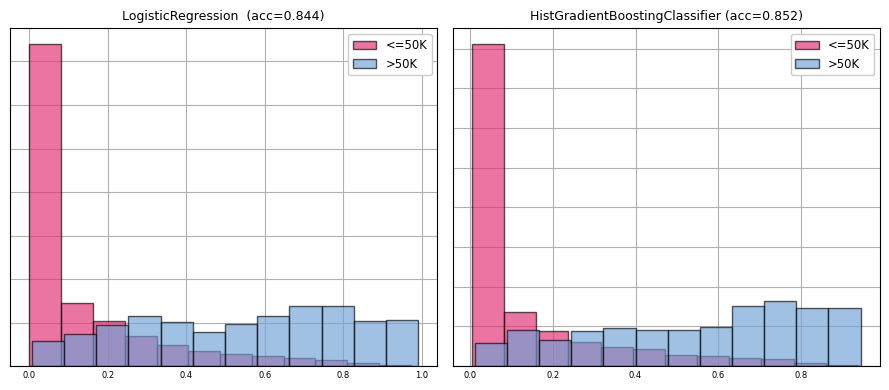
Precision, recall and accuracy are close for each model. We can check if the difference between models is significant using the approach outlined here:
At a significance alpha level at p=0.05, the test concludes that HistGradientBoostingClassifier is significantly better than the LogisticRegression model.
Finally, we can overlay the histograms of model predictions by true class: