The CAS Loss Reserves Database represents a set of triangles intended for use in claims reserving studies. The data includes major personal and commercial lines of business from U.S. property casualty insurers. The claims data comes from Schedule P - Analysis of Losses and Loss Expenses in the National Association of Insurance Commissioners (NAIC) database. NAIC Schedule P contains information on claims for major personal and commercial lines for all P&C insurers that write business in US. The six lines included in this database are: (1) private passenger auto liability/medical; (2) commercial auto/truck liability/medical; (3) workers’ compensation; (4) medical malpractice - claims made; (5) other liability - occurrence; (6) product liability - occurrence.
In this article, a technique to estimate total reserves accounting for correlation between lines of business is introduced. We focus on workers compensation, commercial auto, product liability and other liability data sourced from the CAS Loss Reserves Database. We’ll demonstrate how to account for correlation between lines, and show how changes to the correlation assumption effects the total reserve estimate.
The data can be downloaded from the CAS website directly using data.table’s fread. We perform some preprocessing to normalize column names and assign like columns the same name in each table.
library("data.table")
library("foreach")
library("ChainLadder")
library("ggplot2")

DF1 = fread("https://www.casact.org/sites/default/files/2021-04/wkcomp_pos.csv")  # workers compensation
DF2 = fread("https://www.casact.org/sites/default/files/2021-04/comauto_pos.csv")  # commercial auto
DF3 = fread("https://www.casact.org/sites/default/files/2021-04/prodliab_pos.csv") # product liability
DF4 = fread("https://www.casact.org/sites/default/files/2021-04/othliab_pos.csv")  # other liability

names(DF1) = tolower(names(DF1))
names(DF2) = tolower(names(DF2))
names(DF3) = tolower(names(DF3))
names(DF4) = tolower(names(DF4))

setnames(
    DF1, c("incurloss_d", "bulkloss_d", "accidentyear", "developmentlag"),
    c("incurloss", "bulkloss", "origin", "dev")
    )
setnames(
    DF2, c("incurloss_c", "bulkloss_c", "accidentyear", "developmentlag"),
    c("incurloss", "bulkloss", "origin", "dev")
    )
setnames(
    DF3, c("incurloss_r1", "bulkloss_r1", "accidentyear", "developmentlag"),
    c("incurloss", "bulkloss", "origin", "dev")
    )
setnames(
    DF4, c("incurloss_h1", "bulkloss_h1", "accidentyear", "developmentlag"),
    c("incurloss", "bulkloss", "origin", "dev")
    )
dfList = list(wkcomp=DF1, comauto=DF2, prodliab=DF3, othliab=DF4)
Each dataset contains loss data indexed by grcode, which is a company id. We need to find a company with losses in DF1, DF2, DF3 and DF4. This can be accomplished with the following:
grcodes = Reduce(
    function(v1, v2) intersect(v1, v2),
    lapply(dfList, function(DF) unique(DF[,grcode]))
    )
grnamesDF = unique(
    DF1[grcode %in% grcodes, .(grcode, grname)]
    )
setorderv(grnamesDF, c("grcode"), c(1))
Which yields:
    grcode                              grname
 1:    337                  California Cas Grp
 2:    715               West Bend Mut Ins Grp
 3:   1066                  Island Ins Cos Grp
 4:   1538              Farmers Automobile Grp
 5:   1767                  State Farm Mut Grp
 6:   2143   Farmers Alliance Mut & Affiliates
 7:   5185                    Grinnell Mut Grp
 8:   7080        New Jersey Manufacturers Grp
 9:   9466                      Lumber Ins Cos
10:  10048    Hyundai Marine & Fire Ins Co Ltd
11:  11126 Yasuda Fire & Marine Ins Co Of Amer
12:  13439                 Partners Mut Ins Co
13:  13528              Brotherhood Mut Ins Co
14:  13587                  Chicago Mut Ins Co
15:  14044                Goodville Mut Cas Co
16:  14257                      IMT Ins Co Mut
17:  14370                  Lebanon Mut Ins Co
18:  14508         Michigan Millers Mut Ins Co
19:  15024                Preferred Mut Ins Co
20:  18791                 Virginia Mut Ins Co
21:  23663            National American Ins Co
22:  26433                   Harco Natl Ins Co
23:  28258             Continental Natl Ind Co
24:  35408                  Sirius Amer Ins Co
25:  38300    Samsung Fire & Marine Ins Co Ltd
26:  38733                   Alaska Nat Ins Co
27:  44091 Dowa Fire & Marine Ins Co Ltd Us Br
    grcode                              grname
Let’s go with 1767, which represents State Farm. In the next code block, we subset each data.table to only those records with grcode=="1767", then create runoff triangles for each line of business:
GRCODE = 1767
grList = lapply(dfList, function(DF) DF[grcode==GRCODE,])

triData = foreach(
    ii=1:length(grList), .inorder=TRUE, .errorhandling="stop",
    .final=function(ll) setNames(ll, names(grList))
) %do% {
    currLOB = names(grList)[[ii]]
    DFInit = grList[[ii]]
    DF = DFInit[dev<=max(origin) - origin + 1,]
    DF[,value:=incurloss - bulkloss]
    as.triangle(DF[,.(origin, dev, value)])
}
Triangles for each lob are presented below:
> triData
$wkcomp
      dev
origin      1      2      3      4      5      6      7      8      9     10
  1988  50758  94150 106804 113733 120148 123986 127650 128622 129791 130625
  1989  65423 110204 131509 140383 147011 150266 152264 155017 155979     NA
  1990  68719 141501 165694 181789 189149 194315 196897 201780     NA     NA
  1991  82409 165813 199016 213698 222994 229774 232413     NA     NA     NA
  1992  97138 183451 208163 220275 227404 234320     NA     NA     NA     NA
  1993 106508 167688 195533 212777 220063     NA     NA     NA     NA     NA
  1994  93736 141067 160848 173457     NA     NA     NA     NA     NA     NA
  1995  81309 116739 135447     NA     NA     NA     NA     NA     NA     NA
  1996  66073  92365     NA     NA     NA     NA     NA     NA     NA     NA
  1997  56003     NA     NA     NA     NA     NA     NA     NA     NA     NA

$prodliab
      dev
origin   1   2   3    4    5    6    7    8    9   10
  1988 696 737 881 1002 1379 1451 1741 1814 1818 1850
  1989 428 351 617  718  761  788  797  802  804   NA
  1990  57  77  92  135  197  235  250  263   NA   NA
  1991  23 121 140  141  172  189  190   NA   NA   NA
  1992  48 109 101  107  131  130   NA   NA   NA   NA
  1993 119 133 150  211  278   NA   NA   NA   NA   NA
  1994  21  60  59  100   NA   NA   NA   NA   NA   NA
  1995  57  53  54   NA   NA   NA   NA   NA   NA   NA
  1996  10  11  NA   NA   NA   NA   NA   NA   NA   NA
  1997  20  NA  NA   NA   NA   NA   NA   NA   NA   NA

$comauto
      dev
origin      1      2      3      4      5      6      7      8      9     10
  1988 110231 152848 168137 180062 186150 188142 189352 191307 191867 194000
  1989 121678 158218 176744 188127 192966 196104 199178 199655 200949     NA
  1990 123376 175239 201955 214113 219988 223308 225841 226373     NA     NA
  1991 117457 162601 183338 198607 203398 205870 206957     NA     NA     NA
  1992 124611 166788 189771 201033 206826 212361     NA     NA     NA     NA
  1993 137902 185952 209357 220428 226541     NA     NA     NA     NA     NA
  1994 150582 194528 216205 231077     NA     NA     NA     NA     NA     NA
  1995 150511 194730 215037     NA     NA     NA     NA     NA     NA     NA
  1996 142301 184283     NA     NA     NA     NA     NA     NA     NA     NA
  1997 143970     NA     NA     NA     NA     NA     NA     NA     NA     NA

$othliab
      dev
origin     1      2      3      4      5      6      7      8      9     10
  1988 22417  58806  77536 103003 112976 120070 124641 126954 127444 128036
  1989 24740  55381  76543  97608 113777 124341 126171 128952 132618     NA
  1990 19432  63891  94243 119678 124938 129990 133964 133949     NA     NA
  1991 25821  84453 136275 159204 169820 172446 181744     NA     NA     NA
  1992 38377  98045 138205 154554 171701 177467     NA     NA     NA     NA
  1993 53001 150478 196273 224523 232681     NA     NA     NA     NA     NA
  1994 50848 127767 187297 233255     NA     NA     NA     NA     NA     NA
  1995 59140 149648 215701     NA     NA     NA     NA     NA     NA     NA
  1996 71637 159561     NA     NA     NA     NA     NA     NA     NA     NA
  1997 82937     NA     NA     NA     NA     NA     NA     NA     NA     NA
Next, for each triangle, call the BootChainLadder function (available in the ChainLadder library), running 5000 iterations and retaining only the total IBNR samples from each invocation (discarding IBNR simulations by accident year). We replace simulated values less than or equal to 1 with 1:
ibnrSimsDF = foreach(
    ii=1:length(triData), .inorder=TRUE, .errorhandling="stop",
    .combine="cbind.data.frame", .final=setDT
) %do% {
    tri = triData[[ii]]
    bcl = BootChainLadder(tri, R=5000, process.distr="gamma")
    lobSims = bcl$IBNR.Totals
    lobSims[lobSims<1] = 1
    lobSims
}

# Set names of each column in simsDataDF to associated LOB.
names(ibnrSimsDF) = names(triData)
Inspecting the first 6 records of ibnrSimsDF yields:
> head(ibnrSimsDF)
wkcomp prodliab comauto othliab
1: 213282.5 309.9531 207524.1 836339.0
2: 185281.3 453.1356 228032.9 876116.3
3: 178462.7 263.7076 246759.9 633045.5
4: 204928.1 169.7184 246953.0 641145.2
5: 168382.3 408.6908 213764.4 717701.9
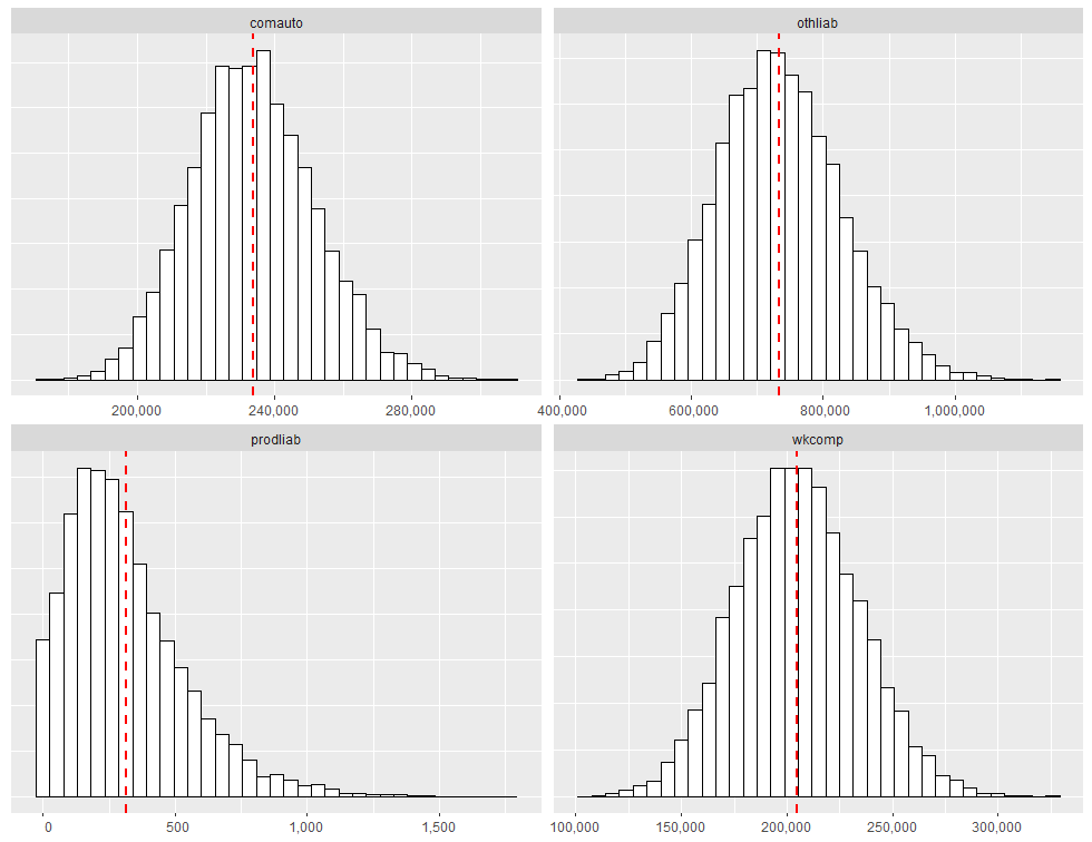
6: 158486.8 194.0509 227606.5 711641.2ibnrSimsDF contains 5000 rows, with the value in each row representing the total simulated reserve need across all accident years for the lob in question. It is possible to produce histograms of the simulated total IBNR using ggplot2. The code that follows generates a faceted quad-plot of the sampling distribution of total IBNR for each lob, with a vertical dashed red line marking the location of the distribution mean. We first transform ibnrSimsDF into a ggplot2-compatible format (which is ggDF):
# Create faceted quad-plot representing sampling distribution of total IBNR.
ggDF = data.table::melt(
    ibnrSimsDF, measure.vars=names(ibnrSimsDF), value.name="ibnr",
    variable.name="lob", variable.factor=FALSE
    )

# Add mean.ibnr for huistogram overlay.
ggDF[,mean.ibnr:=mean(ibnr, na.rm=TRUE), by="lob"]

ggplot(ggDF, aes(x=ibnr)) +
    geom_histogram(bins=35, color="black", fill="white") +
    geom_vline(
        aes(xintercept=mean.ibnr), color="red", linetype="dashed", size=1
        ) +
    theme(
        axis.title.y=element_blank(), axis.text.y=element_blank(),
        axis.ticks.y=element_blank(), axis.title.x=element_blank()
        ) +
    scale_x_continuous(
        labels=function(x) format(x, big.mark=",", scientific=FALSE)
        ) +
    facet_wrap(~lob, scales="free")
Running the code above produces the following exhibit:
Quantifying Total Reserve Variability
If all we are trying to do is determine the expected value of the reserve run-off, we can calculate the expected value for each lob separately and add all the expectations together. However, if we are trying to quantify a value other than the mean (such as the 75th percentile), we cannot simply sum across lines of business. If we do so, we will overstate the aggregate reserve need. The only time the sum of each lob’s 75th percentile would be appropriate for the aggregate reserve indication is when all lines are fully correlated with each other, which is highly unlikely.
To account for correlation between lobs, we rely on the rank correlation methodology described in Two Approaches to Calculating Correlated Reserve Indications Across Multiple Lines of Business. The methodology is carried out through a two-step process:
In the first step, a stochastic reserving technique is used to generate N possible reserve runoffs from each data triangle being analyzed (this is what we have in ibnrSimsDF). In the second step, a correlation matrix is specified, where individual elements of the correlation matrix describe the association between different pairs of lobs. With the correlation matrix \(\Sigma\), carry out the following steps:
Compute the Cholesky decomposition of \(\Sigma\), that is, find the unique lower triangular matrix \(A\) such that \(AA^{T} = \Sigma\).
Compute \(Z = (z_{1}, \dots, z_{n})^{T}\), a vector whose components are \(n\) independent standard normal variates (for our example, \(n=5000\).)
Let \(X = \mu + AZ\). Since \(Z\) represents independent draws from the standard normal distribution, the value of the mean vector \(\mu\) is 0. Therefore correlated random draws are obtained by matrix multiplying \(A\) with \(Z\).
For the correlation matrix, we’ll initially assume no correlation between lobs (all off-diagonal elements=0). Later
we’ll compare estimated reserve need as a function of changing correlation.
The correlation matrix can be initialized as follows:
sigma = matrix(
    c(c(1, 0, 0, 0),
      c(0, 1, 0, 0),
      c(0, 0, 1, 0),
      c(0, 0, 0, 1)),
    nrow=4,
    dimnames=list(names(ibnrSimsDF), names(ibnrSimsDF))
    )
Which looks like the following:
         wkcomp prodliab comauto othliab
wkcomp        1        0       0       0
prodliab      0        1       0       0
comauto       0        0       1       0
othliab       0        0       0       1
The next code block implements steps 1-3:
A = t(chol(sigma))
Z = matrix(rnorm(ncol(A) * 5000), nrow=5000, ncol=ncol(A))
X = Z %*% A
Checking out the first few records of X yields:
> head(X)
         wkcomp    prodliab    comauto    othliab
[1,]  0.2256225  0.66492692  0.8239846 -1.5497317
[2,]  0.1101583  0.60652201 -0.9572046 -0.5200923
[3,] -0.5961369  0.13732270 -1.5355783  1.0622470
[4,]  0.6863108 -1.02719480  0.1086142 -0.4941367
[5,]  1.3918400  0.09805293  0.3412182 -0.1409186
[6,]  0.5547157  1.57012447  0.1263973  0.7135559
For each column in X, we need to obtain the rank of each correlated random draw. This can be accomplished by running:
rankX = foreach(ii=1:ncol(X), .combine="cbind") %do% { rank(X[,ii]) }
colnames(rankX) = colnames(sigma)
Inspecting the first few records from rankX yields:
> head(rankX)
     wkcomp prodliab comauto othliab
[1,]   2971     3758    3975     293
[2,]   2751     3658     856    1493
[3,]   1393     2759     288    4335
[4,]   3785      782    2746    1544
[5,]   4619     2684    3178    2221
[6,]   3569     4687    2784    3866
To prepare for the rank correlation step, we need to order our total IBNR simulations from smallest to largest within each lob column:
# Order total bootstrapped ibnr samples from smallest to largest.
orderedSimsDF = foreach(
    ii=1:length(names(ibnrSimsDF)), .combine="cbind.data.frame",
    .final=setDT
) %do% {
    currLOB = names(ibnrSimsDF)[[ii]]
    sort(ibnrSimsDF[[currLOB]])
}

names(orderedSimsDF) = names(ibnrSimsDF)
Then for each rank in rankX, we lookup the corresponding position-wise element from orderedSimsDF. This ensures that the rank order correlations between lobs are the same as the correlations imposed on the random normal samples. For example, the first row of rankX is:
  wkcomp prodliab  comauto  othliab
    2971     3758     3975      293
Then using orderedSimsDF, we lookup the 2971st element under wkcomp, the 3758th element under prodliab, the 3975th element under comauto and the 293rd element under othliab. This can be accomplished as follows:
# Get correlated IBNR samples.
corrIBNR = foreach(
    ii=1:length(names(orderedSimsDF)), .combine="cbind"
) %do% {
    currLOB = names(orderedSimsDF)[[ii]]
    lobIndx = rankR[,currLOB]
    orderedSimsDF[lobIndx, get(currLOB)]
}

colnames(corrIBNR) = names(orderedSimsDF)
Finally, we sum the correlated samples across lobs, resulting in a vector of values representing the aggregate reserve distribution:
totalIBNR = apply(corrIBNR, MARGIN=1, sum)Percentiles of the aggregate IBNR distribution can be obtained by calling:
> quantile(totalIBNR, c(.01, .25, .50, .75, .99))
       1%       25%       50%       75%       99%
 962340.6 1107900.3 1171348.8 1241553.0 1428743.0
Comparing different values of \(\Sigma\)
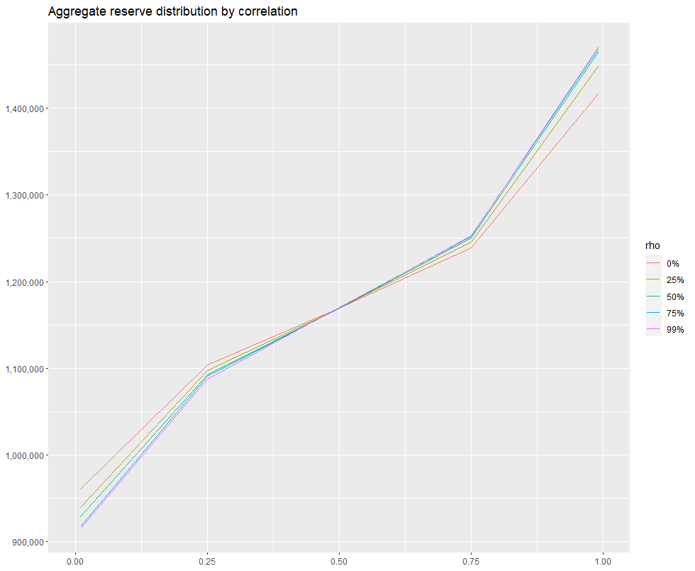
We’ve re-run the procedure described in the previous section for 5 different correlation matrices, assuming 0, .25, .50, .75 and .99 off-diagonal correlation, and combined the results into a single data.table qqDF. I then estimated the 1st, 25th, 50th, 75th and 99th percentile of each aggregate reserve distribution and created an exhibit comparing the distribution of each as a function of percentile. The code used to create the exhibit is given below:
# ------------------------------------------------------------------------
# Assume qqDF contains  1st, 25th, 50th, 75th and 99th percentile of the
# aggregate IBNR distribution for off-diagonal correlation values of
# 0, .25, .50, .75 and .99. The first few records of qqDF look like:
#
#          rho    x         y
#       1:  0% 0.00  871243.8
#       2:  0% 0.25 1107900.3
#       3:  0% 0.50 1171348.8
#       4:  0% 0.75 1241553.0
#       5:  0% 0.99 1428743.0
#
# ------------------------------------------------------------------------
ggplot(qqDF, aes(x=x, y=y)) + geom_line(aes(color=rho), size=.5) +
    scale_y_continuous(
        labels=function(x) format(x, big.mark=",", scientific=FALSE)
        ) +
    theme(
        axis.title.y=element_blank(), axis.title.x=element_blank()
        ) + xlim(0, 1) +
    ggtitle("Aggregate reserve distribution by correlation")
Which produces the following:
By changing xlim(.50, 1) in the code above, we can zoom in on the right-hand side of the distribution:
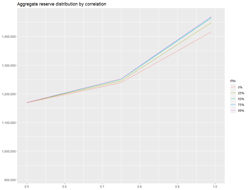
We see that around .50 mark on the x-axis, there is essntially no difference between 0% and 25% off-diagonal correlation assumption. However, as we move right along the x-axis, there’s a greater and greater discrepancy. when x=.99, the difference in the estimated total needed reserve is ~50,000, which represents approximately a 5% difference.
A few take-aways:
If all we are trying to do is determine the expected value of the reserve run-off, we can calculate the expected value for each lob separately then add the expectations together.
If the aim is to quantify a value other than the mean, such as the 75th percentile, we cannot simply sum across the lines of business, as this is akin to assuming full correlation between lines of business, which is unlikely and will overstate the aggregate reserve need.
Off-diagonal correlation values do not need to be the same, but the matrix does need to be symmetric (identical values at \(m_{i,j}\) and \(m_{j,i}\)).